Version: 1.0.4

Twitter Sentiment Classification using Vowpal Wabbit in SynapseML

In this example, we show how to build a sentiment classification model using Vowpal Wabbit (VW) in SynapseML. The data set we use to train and evaluate the model is Sentiment140 twitter data. First, we import a few packages that we need.

import os
import urllib.request
import pandas as pd
from zipfile import ZipFile
from pyspark.sql.functions import udf, rand, when, col
from pyspark.ml import Pipeline
from pyspark.ml.feature import CountVectorizer, RegexTokenizer
from synapse.ml.vw import VowpalWabbitClassifier
from synapse.ml.train import ComputeModelStatistics
from pyspark.mllib.evaluation import BinaryClassificationMetrics
import matplotlib.pyplot as plt

# URL to download the sentiment140 dataset and data file names
DATA_URL = "https://mmlspark.blob.core.windows.net/publicwasb/twittersentimenttrainingandtestdata.zip"
TRAIN_FILENAME = "training.1600000.processed.noemoticon.csv"
TEST_FILENAME = "testdata.manual.2009.06.14.csv"
# Folder for storing the downloaded data
DATA_FOLDER = "data"
# Data column names
COL_NAMES = ["label", "id", "date", "query_string", "user", "text"]
# Text encoding type of the data
ENCODING = "iso-8859-1"

Data Preparation

We use Sentiment140 twitter data which originated from a Stanford research project to train and evaluate VW classification model on Spark. The same dataset has been used in a previous Azure Machine Learning sample on twitter sentiment prediction. Before using the data to build the classification model, we first download and clean up the data.

def download_data(url, data_folder=DATA_FOLDER, filename="downloaded_data.zip"):
    """Download and extract data from url"""

    data_dir = "./" + DATA_FOLDER
    if not os.path.exists(data_dir):
        os.makedirs(data_dir)
    downloaded_filepath = os.path.join(data_dir, filename)
    print("Downloading data...")
    urllib.request.urlretrieve(url, downloaded_filepath)
    print("Extracting data...")
    zipfile = ZipFile(downloaded_filepath)
    zipfile.extractall(data_dir)
    zipfile.close()
    print("Finished data downloading and extraction.")


download_data(DATA_URL)

Let's read the training data into a Spark DataFrame.

df_train = pd.read_csv(
    os.path.join(".", DATA_FOLDER, TRAIN_FILENAME),
    header=None,
    names=COL_NAMES,
    encoding=ENCODING,
)
df_train = spark.createDataFrame(df_train, verifySchema=False)

We can take a look at the training data and check how many samples it has. We should see that there are 1.6 million samples in the training data. There are 6 fields in the training data:

label: the sentiment of the tweet (0.0 = negative, 2.0 = neutral, 4.0 = positive)
id: the id of the tweet
date: the date of the tweet
query_string: The query used to extract the data. If there is no query, then this value is NO_QUERY.
user: the user that tweeted
text: the text of the tweet

df_train.limit(10).toPandas()

print("Number of training samples: ", df_train.count())

Before training the model, we randomly permute the data to mix negative and positive samples. This is helpful for properly training online learning algorithms like VW. To speed up model training, we use a subset of the data to train the model. If training with the full training set, typically you will see better performance of the model on the test set.

df_train = (
    df_train.orderBy(rand())
    .limit(100000)
    .withColumn("label", when(col("label") > 0, 1.0).otherwise(0.0))
    .select(["label", "text"])
)

VW SynapseML Training

Now we are ready to define a pipeline which consists of feature engineering steps and the VW model.

# Specify featurizers
tokenizer = RegexTokenizer(inputCol="text", outputCol="words")

count_vectorizer = CountVectorizer(inputCol="words", outputCol="features")

# Define VW classification model
args = "--loss_function=logistic --quiet --holdout_off"
vw_model = VowpalWabbitClassifier(
    featuresCol="features", labelCol="label", passThroughArgs=args, numPasses=10
)

# Create a pipeline
vw_pipeline = Pipeline(stages=[tokenizer, count_vectorizer, vw_model])

With the prepared training data, we can fit the model pipeline as follows.

vw_trained = vw_pipeline.fit(df_train)

Model Performance Evaluation

After training the model, we evaluate the performance of the model using the test set which is manually labeled.

df_test = pd.read_csv(
    os.path.join(".", DATA_FOLDER, TEST_FILENAME),
    header=None,
    names=COL_NAMES,
    encoding=ENCODING,
)
df_test = spark.createDataFrame(df_test, verifySchema=False)

We only use positive and negative tweets in the test set to evaluate the model, since our model is a binary classification model trained with only positive and negative tweets.

print("Number of test samples before filtering: ", df_test.count())
df_test = (
    df_test.filter(col("label") != 2.0)
    .withColumn("label", when(col("label") > 0, 1.0).otherwise(0.0))
    .select(["label", "text"])
)
print("Number of test samples after filtering: ", df_test.count())

# Make predictions
predictions = vw_trained.transform(df_test)
predictions.limit(10).toPandas()

# Compute model performance metrics
metrics = ComputeModelStatistics(
    evaluationMetric="classification", labelCol="label", scoredLabelsCol="prediction"
).transform(predictions)
metrics.toPandas()

# Utility class for plotting ROC curve (https://stackoverflow.com/questions/52847408/pyspark-extract-roc-curve)
class CurveMetrics(BinaryClassificationMetrics):
    def __init__(self, *args):
        super(CurveMetrics, self).__init__(*args)

    def get_curve(self, method):
        rdd = getattr(self._java_model, method)().toJavaRDD()
        points = []
        for row in rdd.collect():
            points += [(float(row._1()), float(row._2()))]
        return points


preds = predictions.select("label", "probability").rdd.map(
    lambda row: (float(row["probability"][1]), float(row["label"]))
)
roc_points = CurveMetrics(preds).get_curve("roc")

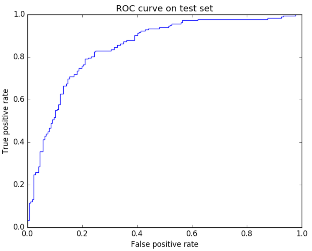
# Plot ROC curve
fig = plt.figure()
x_val = [x[0] for x in roc_points]
y_val = [x[1] for x in roc_points]
plt.title("ROC curve on test set")
plt.xlabel("False positive rate")
plt.ylabel("True positive rate")
plt.plot(x_val, y_val)
# Use display() if you're on Azure Databricks or you can do plt.show()
plt.show()

You should see an ROC curve like the following after the above cell is executed.

Twitter Sentiment Classification using Vowpal Wabbit in SynapseML

Data Preparation​

VW SynapseML Training​

Model Performance Evaluation​

Data Preparation

VW SynapseML Training

Model Performance Evaluation